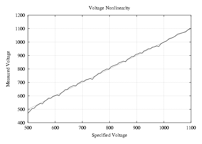
There were three problems associated with using the high voltage to select energies to measure. First, the high voltage setting selected from the controls did not match the actual high voltage obtained as shown in the following plot.
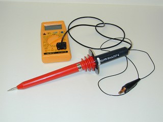
The gray line shows the ideal linearity and the black line shows the actual linearity. While overall linearity is acceptable, there are local variations in the voltage that would produce somewhat confusing spectra as energies can appear out of order. To rectify this, a Fluke 80K-40 high voltage probe (shown below) was used with a cheap 10 Mohm input impedence DVM to measure the actual voltage produced at each setting. These measured voltages were used in plotting the spectra.
A second problem was the high voltage setting did not permit enough resolution to obtain a good spectrum. The voltage is controlled internally via an 8-bit digital to analog converter. This yields 256 possible voltage settings between the 500 and 2450 volt limits so the settings are about 7.6 volts apart. In this case, the voltage setting was limited to the range 500-1100 volts yielding 76 steps. To increase the resolution, the high voltage was adjusted slightly using the available trimming potentiometers between runs. For example, the first run was made after calibrating the high voltage to factory specifications. This involved setting the potentiometers so the displayed and measured voltages matched at 607 and 1800 volts. For the next run, the voltages were tweaked so the actual voltages were 611 and 1804 volts. By making many, many runs in this manner, varying the actual voltages slightly each time, a final resolution of 1 volt was obtained. The actual voltage range measured by the DVM was 465-1112 volts for 648 discrete settings.
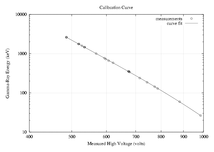
The biggest problem with using high voltage to select the energy is the gain of a PMT is a strong function of this voltage. To make any sense of the measurements, a relation between the applied voltage and the corresponding gamma-ray energy had to be developed. By identifying the energies of the prominent peaks in each spectrum and plotting them against the HV values used to produce them, a curve fit was developed to show the relationship. The resulting calibration curve is shown below.
| Return to Home Page | Latest update: July 18, 2004 |