
Below are two plots of the light pollution near where I live. The first includes the area around Santa Fe, Texas including parts of League City, Kemah, Dickinson, Texas City, La Marque, Hitchcock and Alvin.
The yellow squares of varying intensity represent the level of background light visible at the zenith. Brighter yellow corresponds to brighter skies. The brightness is given as the equivalent brightness of a star in each square arcsecond of sky required to produce the same overall brightness level. Star magnitudes are logarithmic with each decrease of 1 magnitude equal to approximately a 2.5x increase in light. Low numbers thus correspond to bright skies. All measurements were made on clear nights when the moon did not interfere with the readings.
The data was recorded using a Unihedron "Sky Quality Meter". This hand-held device measures the visual magnitude of the sky in a roughly 40 degree half-angle cone. To obtain the data, the "Sky Quality Meter" was used to record the brightness through the open sunroof of a moving car at approximately 20 second intervals. GPS data was recorded at the same time so the brightness readings could later be tagged to their location. On the plot above, the thin gray lines represent the routes taken during data measurement as recorded by the GPS receiver. A few of the roads these routes included are labelled.
To make the color contours, the Santa Fe area was broken into a 32x32 grid. The brightness value for each grid cell was set equal to the maximum (darkest) reading from all data points that happened to fall in the cell. Ideally the meter would have had an unobstructed view of the sky. In many cases, however, the field of view contained tree branches or power lines or light from streetlights hit the front of the unit. Any of these would lead to artificially bright readings. By using only the darkest reading in each cell it is hoped the readings correspond to times when no such contamination of the data occurred.
To account for night-to-night variations in sky brightness due to haze etc., values of brightness from each night were compared to each other where the routes passed through common cells. The median of the differences across all such cells were used to adjust the data to a common datum. This was not totally effective in removing these differences. Part of the problem was the brightness at a given location was seen to vary throughout the data taking period each night. No attempt has been made yet to correct for this effect.
The second plot shows similar brightness contours taken farther north in the Clear Lake City, Texas area. This data was taken several years ago before the Unihedron meter was available.
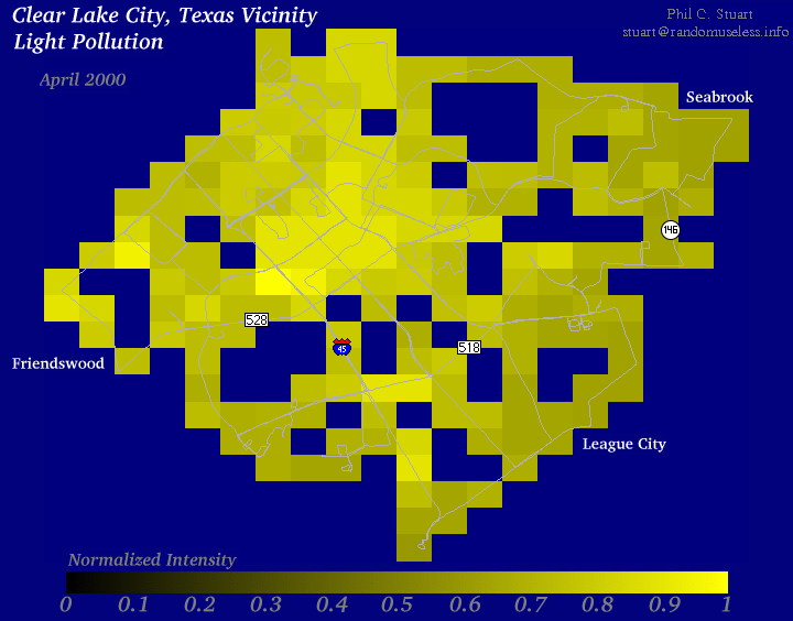
These measurements were made with a modified Connectix QuickCam grayscale camera hooked to a PC laptop running Linux. The camera modification involved removing the camera components from the plastic "eyeball" enclosure and installing them in a small cast aluminum project box. A C-CS lens adpapter was expoxied to a hole in the front of the box to allow C-mount lenses to be used instead of the standard QuickCam lens. The infared blocking filter was also removed.
The QuickCam is capable of rendering a scene with 64 shades of gray. Using an f/1.3 lens and the maximum exposure time yielded sky images with an average gray level around 20.
The camera was mounted in the console of my car. A 12mm lens was used which had a sufficiently small field of view that the camera could get an unobstructed view up through the open sunroof.
The software used to make the readings was a slightly modified version of the free "xqcam" program by Paul Chinn. This program can continuously take images displaying them in an X-window. Two code modifications were made as briefly described below.
1. Since the exposure time is long (approx 1 second) the thermal signal builds up in the CCD chip causing an intensity gradient from top to bottom across the image. To minimize this effect, pixels at the edge of the image that are shielded from light are used. Since the complete exposure these pixels contain is due to thermally generated electrons, the median of each row was subtracted from the imaging pixels on the row to remove the thermal effect. 2. Since only the sky background brightness was desired, the median of the imaging pixels was calculated after the above correction. This value was written, along with the time, to the screen and to a file. This is the brightness value visible in the image above.
To figure out where each brightness value was measured, a GPS receiver was used. Ideally, the GPS reciever would have been used to trigger the QuickCam at a fixed time interval so the image and location would have been recorded simultaneously. Since my receiver is an OEM board requiring external power etc., I simply used the setup I built for my radioactive vacation in 1998.
The procedure used to take the measurements is as follows.
1. Start the GPS recorder. It is set to output an NMEA sentence containing the time, longitude, latitude, and number of satellites. The output interval is 10 seconds. 2. After the GPS locks on the satellites, record the time according to the laptop and the GPS receiver. This will be used later to adjust the QuickCam image times to the correct time. 3. Move to a starting location common to all the runs and start the camera. By always starting data taking at the same location, night-to-night variations in brightness can be corrected for. 4. After several brightness values have been stored at the starting location, the desired route is driven.
Once data collection is complete, the plotting procedure is:
1. Shift the image times by the offset from the GPS reciever. 2. Linearly interpolate the image times from the GPS data to find the location where each image was taken. 3. Scale the brightness values so the starting values at the known location are always the same value. 4. Calculate the max and min longitude and latitude for all images. 5. Break the longitude/latitude region into 20 bins each way. 6. Loop through the images binning them into the longitude/latitude bins. As with the Santa Fe data, only the darkest readings were kept for each bin. 7. Plot the bins as shown in the image above. Since the frames were taken automatically there was a much better chance of trees etc. being in the field of view during a reading. For this reason, a cell was only plotted if there were at least 5 readings inside it. This minimized the possibility that all of the available readings were bad.
Note that, unlike the newer Santa Fe data, these older measurements are linear with sky brightness. For this reason and because the relationship between the older readings and light intensity are unknown, the color bars on the two plots are unrelated.
Since my GPS setup also contains a Geiger Counter, radiation levels were recorded as well. The sample size was much too small, however, to yield anything more than random noise.
To find out more about light pollution check out the web site of the International Dark-Sky Association. They have tips on modifying your lighting to enhance security and reduce energy use while helping to preserve the night skies.
| Return to Home Page | Latest update: March 5, 2006 |